Who switched the light on?
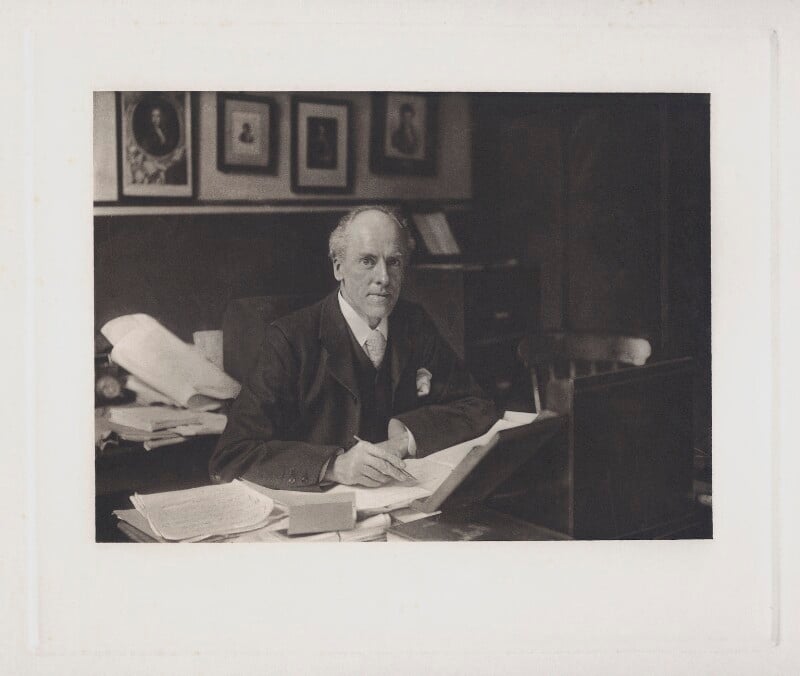
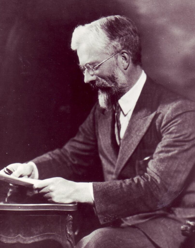
In the history of statistics, the period from 1885-1935 is known as the ‘Statistical Enlightenment’ (Stigler, 2010). The outstanding contribution of two individuals from this period – Karl Pearson and R. A. Fisher – was the prime source of light that ‘pierced the darkness’. Try imagining a world of statistics without correlation or regression or the sampling distribution or hypothesis testing or randomisation and you begin to appreciate Pearson’s and Fisher’s role. But to understand why their work matters so much it’s not enough to simply produce a long list of their many contributions; we need to know where their work fits in in the evolution of statistics and how it helped statistics adapt to meet the changing needs of science and the modern world.
Statistics
Today, we live in a society that counts everything and relies heavily on numbers. Statistics plays an important role in the study of the collection and mathematical analysis of data. But unless you are aware that there was a time when statistics were not numbers you may never have wondered how this came to be. The eighteenth-century German tradition of Statistik, which gave us the word statistics, insisted on verbal descriptions of the state. Its English rival, the political arithmetic of the late seventeenth and eighteenth centuries (which became social statistics in the nineteenth century) compiled lots of numerical data but didn’t analyse them mathematically. A mathematical theory of probability developed separately to tackle insurance problems and as a way of measuring risk in situations such as gambling. Probability was part of the work of mathematicians who mostly worked with abstract examples and without large quantities of statistical data.
The nineteenth century saw an unprecedented growth in the large-scale collection of data in a variety of different intellectual fields. This prompted statisticians to ask new, deeper questions about the meaning, structure and relationships in the data. And as the quantity and complexity of the data grew, mathematics was increasingly seen as the way to handle things. By the early twentieth century mathematical analysis, including probabilistic analysis, were an indispensable part of statistical practice. This was largely due to the contributions of Pearson and Fisher. Pearson’s pioneering work on asymmetrical distributions benefitted greatly from the method of moments while his work on regression and correlation advanced through the introduction of matrix algebra to statistics. The pressing problems of estimation and sampling with which Fisher dealt found powerful solutions in n-dimensional geometry and the method of maximum likelihood. But Pearson and Fisher did more than just add to the mathematics of statistics – the mathematisation of statistics helped turn statistics from a ‘Gradgrindian’[1] obsession with the collection of data about anything and everything into a universally applicable method that can be used to advance all of science.
Statistical data
Throughout its history, statistics has dealt with different kinds of data and has evolved through its attempts to solve the questions that these different kinds of data presented.
Up to the late nineteenth century, statistical data were mostly social data. Working with social data stimulated the development of the statistical table and graphical visualisation methods, such as the pie and bar charts invented by William Playfair in the late eighteenth and early nineteenth centuries. Later on, a desire to use empirical evidence to solve social problems stimulated an unprecedented large-scale collection of social data.
However, it was working not with social, but with astronomical data in the late eighteenth century that spurred the advance of more sophisticated, mathematical, statistical analysis. This was largely because inaccurate and imprecise measurements were a huge problem when working with natural scientific data. So the theory of probability, first called the theory of errors, developed in mathematical astronomy as a way of improving measurement procedures.
Pearson’s work brought together the social statisticians’ desire for lots of data and the astronomers’ desire for better analysis. His work marks an important realisation that natural science needs statistical data to a much greater degree than was previously recognised; and that the calculus of probability couldn’t release its full potential in the field of abstract mathematics – it, too, needed data. It was this way of thinking which was already present in Francis Galton’s work from the 1870s and 1880s that made possible bivariate and multivariate analysis. And it is through this way of thinking that statistical data acquired a new property – variation. With Galton and Pearson, variation came to be understood as a property of statistical data, not as a property of the measurement process, as it has previously been seen.
What comprised statistical data changed again with Fisher. Up to the early twentieth century, statistics developed for the purpose of analysing large amounts of observational data. But, as the century developed, a new generation of statisticians, which included W.S. Gosset and Fisher, worked in a different context – experimental science. Fisher’s work helped statistics evolve into a powerful method for designing experiments and analysing experimental data. With Fisher, experimental data became statistical data. Statistical control could now replace physical experimental control when the latter was not possible. Statistics provided universal rules, such as randomisation, null hypothesis testing and significance, with which experimental practice could proceed in a systematic and replicable manner.
Statistical explanation
During most of the nineteenth century, statisticians believed that studying statistical data will help them understand the causes or laws that produced these data. Statistical explanations were still deterministic.
In the work of Karl Pearson statistical explanations changed from being about causes to being about variation and probability. With Pearson, to statistically explain something meant to explain, using probability, how this thing varied. This new type of explanation was made possible by Galton’s invention of regression and correlation, and Pearson’s subsequent development of these. Pearson clearly understood the magnitude of this change: ‘Up to 1889 men of science had thought only in terms of causation; in future they were to admit another working category, that of correlation’ (Pearson, 1924: 1).
With Fisher, statistical explanation underwent further changes. To simplify the analysis of variability, which in Pearson’s time relied on the measurement of correlations, Fisher, in 1918, introduced the concept of variance. Later he introduced a technique for the analysis of variance, ANOVA, which is one of the most commonly used bases for statistical tests.
Hypothesis
Whatever the mechanics of statistical explanations – whether they are causal, correlational or use variance – statistical explanations are particular statements, or hypotheses.
The Scientific Revolution of the seventeenth/eighteenth centuries brought us a specific understanding of hypotheses – as something which approximates reality and which scholars test through experiment or observation using empirical evidence (Shapiro, 1983). This was closely linked to the concurrent emergence of the understanding that much of human knowledge, and much of the knowledge produced by the New Science, was probabilistic.
However, despite the early parallel emergence of the modern concepts of hypothesis and probability, up to the late nineteenth century the testing of scientific hypotheses using mathematical probability was rare (John Arbuthnot’s 1710 An Argument for Divine Providence could be considered an exception). Many scientific hypotheses could be tested experimentally or with the help of traditional, non-probabilistic, calculus; while the calculus of probability was used to answer statistical questions like ‘How likely is X?’ or ‘What’s the average of X?’ which did not necessarily require the testing of a specific hypothesis.
When Pearson began his work in statistics in the 1890s, the question ‘How likely is X?’ had already been giving way to another question – ‘How likely it is that X is due to chance?’ This second question requires the setting of a hypothesis because a chance mechanism is brought into play – we hypothesise that the observed data is due to chance.
Pearson’s work on the χ2 tests made it possible to adequately answer this question by allowing us to measure how well an observed distribution fits an expected or hypothetical distribution. However, these tests were isolated contributions that stemmed from, and were limited to, the specific problems that Pearson was trying to solve. It is also important to note that Pearson himself did not use the terms ‘hypothesis’ and ‘test’ to describe his work on the χ2. At this early stage statistics lacked a framework for the designing of studies and for the testing of scientific hypotheses.
Fisher’s work established this robust framework for testing – the terms ‘test of significance’ and ‘statistical significance’ and the rules of hypothesis testing based on the notion of a null hypothesis and nominal levels of significance, such as 5%, are all due him. Thus it is largely due to Pearson and Fisher that we understand statistical hypotheses as hypotheses relating to the population from which the empirical evidence tested is drawn and that we can treat scientific hypotheses as statistical hypotheses.
Distributions
The concept of a statistical distribution has also undergone changes in which Pearson and Fisher played an important part. Up to the late nineteenth century, the Gaussian (bell-shaped) distribution reigned supreme. Social statisticians, like Quetelet, used it to analyse mean values and saw everything else that fell under the curve as redundant information, similar to the way dispersion was perceived in astronomy where it was a product of erroneous or imprecise measurements.
Where attention was paid to dispersion, social statisticians were fascinated by just how many social phenomena apparently fit a bell-shaped curve, an erroneous conclusion they reached due to a lack of rigorous checks of the shape of empirical distributions (Stigler, 1986: 330).
Pearson was the first to question the seemingly ubiquitous power of the Gaussian distribution to describe empirical data and offer alternative solutions. Between 1895-1914, he described a whole family of asymmetrical distributions, including the χ2 distribution used in Pearson’s goodness-of-fit test. As statistical analysis embraced dispersion and welcomed asymmetrical distributions, Pearson popularised the rather unexciting term ‘’normal’ to describe the Gaussian distribution.
Pearson’s distributions were real things in two senses. First, as David Salsburg (2002) argues, with Pearson reality itself became a distribution. For instance, if we could measure the beak lengths of all the finches in a given species, the distribution function of those beak lengths would have its four parameters (mean, standard deviation, skewness and kurtosis) and they would be the beak length of the species. Second, Pearson’s distributions were distributions of real things – crabs, people, skulls etc. And this is the way it had been in statistics. But not for long, since Fisher touched everything that Pearson (and those before him) worked on, including distributions.
It started with a small but crucial problem: How could you know that the estimates you make based on observed data are accurate and precise, especially if you use small samples of data as Fisher did (with a large sample, we could be a bit more relaxed, as Pearson was)? To solve this problem, Fisher used the mathematical concept of the Central Limit Theorem which states that the mean of a great number of independent, random observations is approximately normally distributed – the greater the number of observations, the closer the approximation. So, Fisher reckoned, if you make sure the sample you collected is random, then you can assess the reliability of the estimates with reference to an imaginary distribution of an infinite number of random samples similar to yours because that imaginary distribution, following the Central Limit Theorem will approximate the normal distribution, as the sample size grows. In less than a century, the evolutionary tree of statistics grew two new branches – asymmetrical distributions which help us capture reality more accurately; and sampling distributions which are the bedrock of statistical inference.
Inference and probability
From its emergence in the seventeenth century the concept of probability was seen as necessary and useful because of humankind’s limited capacity for knowledge. Only an infinite intelligence could have perfect knowledge. We humans would have to make do with knowledge defined by moral certainty – high degree of probability that is short of mathematical certainty but allows for action – and use probability to quantify degrees of certainty, or belief.
Inference from data was understood as the revision of knowledge in the light of relevant new information. This is well-illustrated by the work of Thomas Bayes who in the mid-eighteenth century gave us a mathematical formula which uses probability to helps us combine existing knowledge with new evidence in order to arrive at a more enhanced, better state of knowledge.
Doubts that probability could be a measurement of something else, not (or apart from) degrees of belief, and that inference may be something else, not merely revision of old knowledge, began to creep in in the second half of the nineteenth century: ‘Does probability exist in the things which are probable or in the mind which regards them as such?’ William Stanley Jevons asked in 1874 (Jevons, [1874] 1913: 197). These doubts became more acute towards the late nineteenth century as probabilistic statistical analysis entered new fields such as biology where existing knowledge about biological populations was scarce. In such situations, in which assumptions about a prior probability (or a population) couldn’t be made or could be made only speculatively, using a Bayesian approach to make inferences could be misleading.
Pearson had reservations about Bayesian inference but didn’t provide an alternative analytical solution. It could be argued, however, that he found a practical solution for his own purposes – collect large samples of data. This produced estimates that were accepted as sufficiently good to be used in analysis as if they were describing the population, and not merely the sample data.
But Fisher was in a different situation. Pearson’s ‘large samples solution’ didn’t work for him, since he dealt with small samples. Also, Fisher was strongly against the common practice of assigning equal prior probabilities to events in situations in which it wasn’t clear if one probability was any better than another (i.e. when prior knowledge was scarce). He offered an alternative to Bayesian inference which is now known as frequentist inference. This new set of logical principles for making inferences from a sample was based on the concept of probability as objective frequency (not as degrees of belief). This understanding of probability – as a characteristic of the experimental or testing process itself, rather than as an assessment of the credibility of evidence – had first been described in the 1840s, but Fisher was the first to use it to form a coherent theory of inference.
Samples and sampling
The evolution of samples and sampling played an important role in this new theory of inference because frequentist inference is based on the distribution of random samples. Sampling came under spotlight relatively late – up to the 1890s, statisticians thought the key to better statistics was ‘Let’s gather more data!’ as opposed to ‘Let’s develop a more sophisticated mathematical theory of statistics!’. Sampling meant that statisticians should be content with using less data and it was difficult to imagine how this could improve things for two reasons.
First, in the nineteenth century the populations studied were populations of real people. In practice it might have been difficult to collect demographic data about the whole British population; but, it was thought, in principle, given the time, effort and adequate equipment, these population data could be collected. So this remained the goal.
Another reason why sampling was largely inconceivable up until the late nineteenth century was that any early attempts at sampling would have needed good population data to check if using samples really worked – these data were not yet available.
Things changed when the focus of statistical enquiry shifted to also cover biological populations. While it might not be difficult to conceive of the possibility of measuring the whole population of a country, it is much more difficult to conceive of measuring, even in principle, the whole population of finches or spider crabs. When populations became too big (and too expensive) to measure, then statistical workers didn’t have a choice but to turn to sampling.
For Pearson, samples were the practical norm and he worked most often with large samples. He didn’t distinguish, theoretically, between samples and populations. Fisher, again, was different. With limited data and unlimited imagination he laid the foundations of the statistical analysis of small samples, introducing a formal distinction between sample statistics and population parameters, defining the sampling distributions of many important statistics and devising a mathematical theory of estimation. Fisher’s work brought in the realisation that sampling can be beneficial when put to inferential use.
Inference relies on random samples. While random sampling was evolving in the hands of many statistical workers in the early twentieth century, Fisher transformed randomness from a property of the sampling process to a requirement for experimental design. Statisticians could now use the probabilistic inference to analyse and design both observational and experimental studies.
Subjects, like species, evolve by responding to change. In their work, Pearson and Fisher responded to the changing needs of science and society, making contributions that established the mathematical foundations of modern statistics, developing the terminology, theory and techniques of the subject and broadening the scope of its application. But more than anything else, Pearson and Fisher showed how readily statistics can adapt to humankind’s never-ending search for knowledge.
Note
I wrote the first draft of this essay in 2020. To prepare the text, I studied Karl Pearson’s and R. A. Fisher’s published works. I also benefitted from reading the works of Joan Fisher Box, Ian Hacking, Nancy Hall, Eileen Magnello, Egon Pearson, Theodor Porter, David Salsburg and Stephen Stigler. Thank you to Ronald Wilson, John MacInnes and Lindsay Paterson who read a draft of this essay and made valuable suggestions for improvement.
Bibliography
Jevons, W.S. (1913 [1874]). The Principles of Science: a Treatise on Logic and Scientific Method. London: Macmillan and Co.
Pearson, K. (1924). The Life, Letters and Labours of Francis Galton, vol. II. Cambridge: Cambridge University Press.
Salsburg, D. (2002). The Lady Tasting Tea: how Statistics Revolutionized Science in the Twentieth Century. New York: Henry Holt and Company.
Stigler, S. M. (1986). The History of Statistics: The Measurement of Uncertainty before 1900. Cambridge, Massachusetts and London: Harvard University Press.
Stigler, S. M. (2010). ‘Darwin, Galton and the Statistical Enlightenment’, Journal of the Royal Statistical Society A, 173(3): 469-482.
[1] Reference to Thomas Gradgrind, a grotesque character and superintendent in Dickens’s novel Hard Times (1854). The term ‘Gradgrindian’ is used to describe someone who is ‘hard and cold, and solely interested in facts’. Source: OED.