Paintings and charts
Paintings and charts have a lot in common. Like a painting, a statistical chart can be visually appealing, clear and with a good composition (or not!). Both paintings and charts convey information and can arouse emotions and stir the imagination. Understanding the meaning of both requires paying careful attention to detail and some knowledge of context.
However, because charts are a form of scientific illustration, they differ from paintings in several important ways. While the meaning of a painting is usually wide open to interpretation, a chart normally has a very specific meaning. Good charts communicate the meaning of data as unambiguously as possible. Unlike paintings, charts have a very specific purpose – to represent data accurately, clearly and concisely. And while there’s plenty of room for creativity in the art of chart composition, unlike artists, all data scientists or data journalists must follow some commonly agreed standards.
Why bother with charts?
Take this example from Our World in Data:
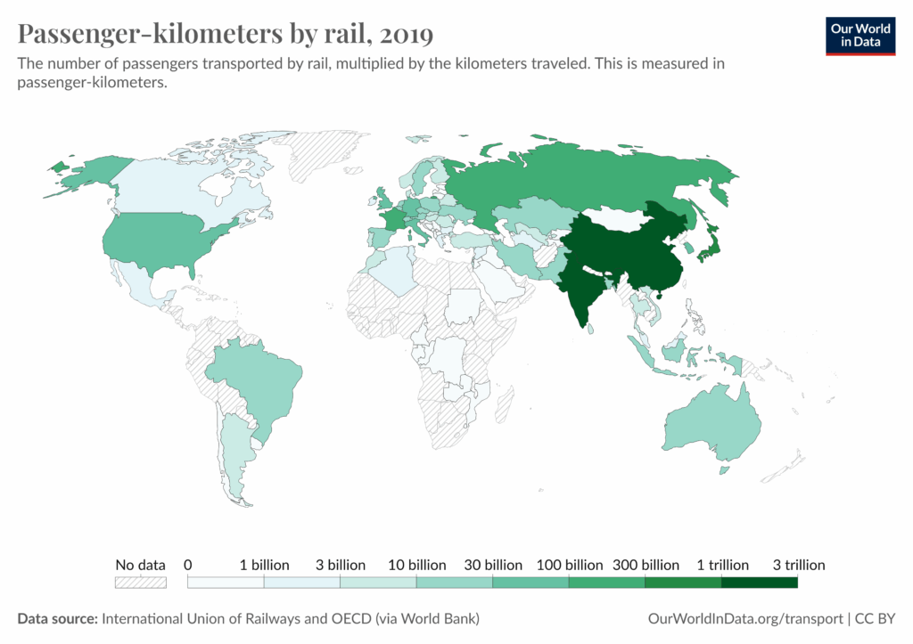
It shows the number of passengers transported by rail in 2019, multiplied by kilometres travelled. This metric, called passenger kilometres, enables us to measure how many people travel by rail in a country and how long a distance they travel. The chart has a specific and unambiguous message – it tells us how well countries are connected by a railway network and illustrates this by using data on both countries’ rail passenger capacity and countries’ capacity to carry rail passengers a long distance. It uses colour to show us how countries differ – the darker the shade of green, the better connected by rail the country is.
When done well, like the example above, charts can help us explore data, especially large amounts of data. There’s no other way, for example, to get a quick and clear view of railway capacity of countries across the world. Charts can also help us formulate questions – e.g., Why are China, India and Russia top of the list? Charts can help us make arguments. For instance, a passenger-kilometres chart can be helpful in making a case about the state of the economy in China, India and Russia. Last but not least, charts can help us communicate knowledge accurately, quickly and effectively to a wide audience.
The beginnings of data visualisation
Although graphing data sounds like a very useful thing to do, charts of the kind that we are used to nowadays are a very recent invention. This is another important way in which paintings and charts differ – archaeologists have found representational art dating back to ca. 30,000, even ca. 44,000 years ago while, in contrast, the first known statistical chart dates back to … 1644 AD!

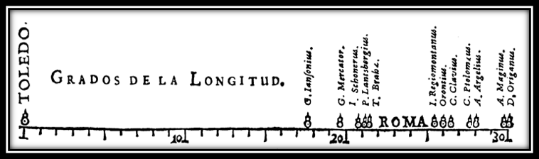
The chart was drawn in 1644 by the Flemish astronomer to the Spanish court, Michael Florent van Langren. It shows 12 different estimates of the distance between Toledo in Spain and Rome in Italy, measured in degrees longitude and ordered from the smallest to the largest estimate. Longitude, or distance east-west from the prime meridian, was difficult to measure up until the mid-18th century, for a variety of reasons – hence the great variation in estimates displayed in van Langren’s chart. Looking at the chart, we see that van Langren has placed Toledo on the prime meridian of 0 degrees. The names that you see vertically along the x-axis are the names of the different astronomers who provided the different estimates.[1]
‘[…] whatever can be expressed in numbers, may be expressed in lines’
The first systematic attempts to visualise data were made in the late eighteenth century. The person who contributed more than anybody else at the time to show how charts can be used in data analysis and to popularise their use was William Playfair (1759-1823). It was Playfair who invented many of the currently used graphical forms (the pie chart) and improved others (the line chart, the bar chart).
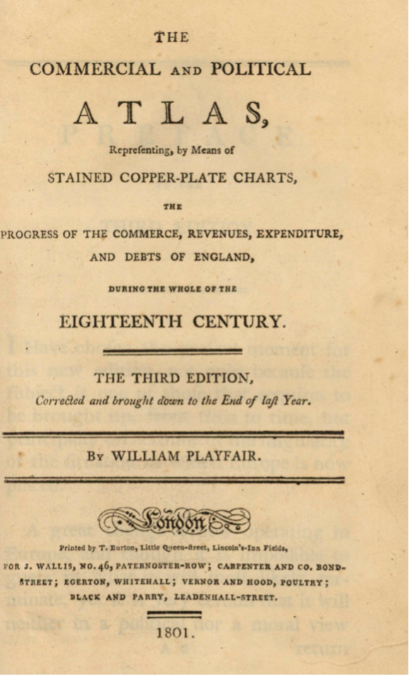
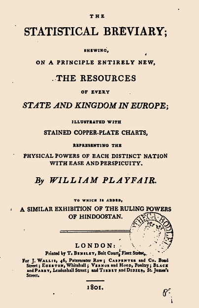
Playfair was guided by the principle, which he learnt as a child from his elder brother, the mathematician John Playfair, that ‘whatever can be expressed in numbers, may be expressed in lines’ (Playfair, 1805: xvi). Thinking in this way was a real breakthrough because it meant that anything that could be measured numerically could be mapped on a 2D space, just like distance between two cities on a map. Using this analogy, Playfair explained that a map can be devised showing any quantities, not just longitude and latitude measured in degrees. That’s why he called his first major book on this topic The Commercial and Political Atlas (1786), even though it didn’t contain any geographical maps. The Atlas as well as his other major work, The Statistical Breviary (1801), contained graphs of actual data on, e.g., trade, commodity prices and country revenue.
Playfair’s line charts
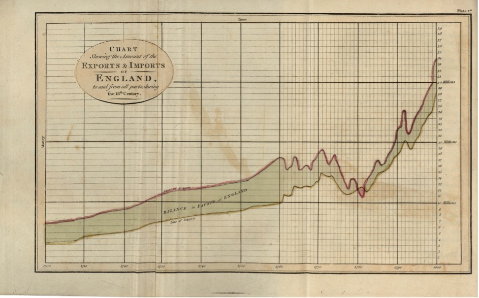

Figures 6 and 7 show two line charts from Playfair’s The Commercial and Political Atlas (1801 [1786]). Figure 6 shows how the amount of exports and imports in England changed during the eighteenth century. The yellow line denotes imports and the red line denotes exports. Almost throughout the entire 18th century, England was exporting more than it was importing.
Figure 7 shows how the price of flour fluctuated in the 1790s. In total there are 44 line charts in Playfair’s Atlas. These charts were the first to employ colour, and also area, to indicate different quantities. Playfair’s charts were not always precise; however, they showed that graphing data could be very useful in examining relationships between variables – in his case time and money. Playfair’s work marks the birth of what we call ‘relational graphs’.
The first modern bar chart
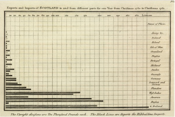
Most of the charts in Playfair’s Atlas were based on longitudinal data from records dating back to the year 1700. These data were available for England but not for Scotland. As a result, to depict the exports and imports of Scotland, Playfair couldn’t use the line graphs which he used to present the England data. Instead, he depicted the little data that he had about Scotland in a different graphical form which has come to be known as the bar chart. Strictly speaking, Playfair didn’t invent the bar chart – a version of a bar chart had been used by the polymath Joseph Priestley several decades earlier. However, in Playfair we see the bar chart in its modern form for the first time. One of the things that distinguishes Playfair’s chart from the earlier form used by Priestley, bringing it closer to the modern form, is the fact that he ordered the bars by length, starting at the bottom, with the country with which Scotland traded the most – England. This sounds obvious to us, but back in those days it wasn’t an obvious thing to do.
The first pie charts
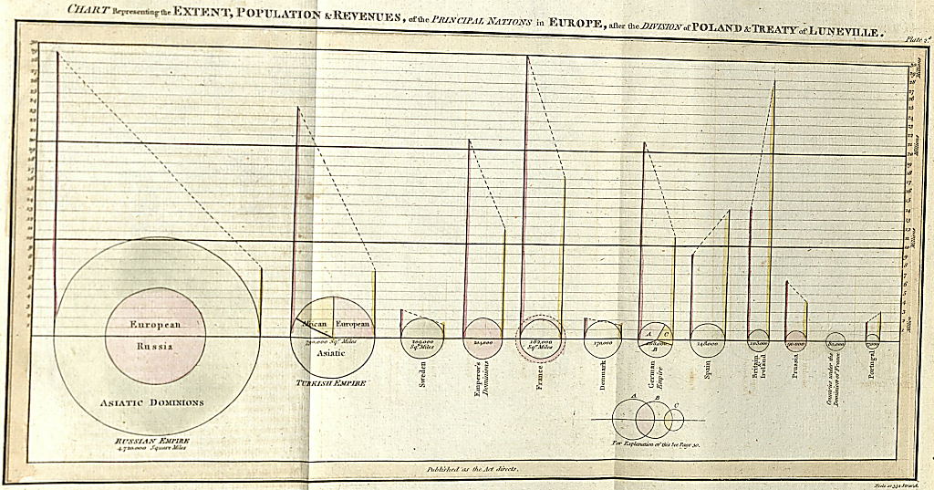
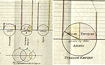
Figure 9 shows another chart by Playfair that summarises statistical information about several European countries. Here Playfair used area to depict the size of a country and colour to indicate the continent or continents where each country had territories. The red line on the left side of each circle area represents the country’s population in millions; the yellow line on the right of each circle depicts countries’ tax revenue in millions of pounds sterling. For example, looking at the first item on the left hand-side of the chart, we see that Russia has the greatest area, with a population of about 25 million spreading across two continents, Europe and Asia, and a tax revenue of about 7 million. To represent how the Turkish empire was split between three continents (Figure 10 right), Playfair invented the modern pie chart. He used another pie chart (Figure 10 left) to show the German empire was split between three powers (‘Austria’, ‘Prussia’ and ‘Other German Princes’). The red part shows how much of the empire belonged to the house of Austria; the yellow portion represents what the Prussian part and the green – what remained to the other ‘Princes’.
If you’d like to learn more about the history of statistical charts and about Playfair’s work, the sources listed below are a great place to start!
Bibliography
Friendly, M., and Wainer. H. A History of Data Visualization and Graphic Communication (Cambridge: Harvard University Press, 2021).
Friendly, M. et al. ‘The First (Known) Statistical Graph: Michael Florent van Langren and the “Secret” of Longitude’ The American Statistician, 64(2010), 174–184.
Langren, M. F. La verdadera longitud por mar y tierra, 1644.
Playfair, W. The Commercial and Political Atlas (London: Printed by T. Burton, 1801).
Playfair, W. The Statistical Breviary (London: Printed by T. Bensley, 1801).
Playfair, W. An Inquiry into the Permanent Causes of the Decline and Fall of Powerful and Wealthy Nations. Designed To Shew How The Prosperity Of The British Empire May Be Prolonged (London: Printed for Greenland and Norris, Booksellers: 1805).
Tufte, E. R. The Visual Display of Quantitative Information (Cheshire, Conn.: Graphics Press, 1983).
[1] Now we know that the real longitude between the two cities is about 16 degrees – most of the early estimates were way off! For more details, see Friendly et al, 2010.
[2] Playfair, 1805, p. xvi.